Loan Default Prediction Machine Learning Project
This is an exploratory project for me to apply different Machine Learning (ML) models and techniques and have a better understanding of how each of them work and interact with the data:
- Feature Engineering
- One-hot encoding for categorical features
- Normalization/standardization
- Imputation
- Feature expansion
- Feature dimension reduction:
- Feature hashing
- Feature selection
- Principal component analysis
- Decision Tree Feature Importance
- Feature discretization with Random Forests and Gradient-Boosted Decision Trees
- Machine Learning Models:
- Logistic Regression
- Decision Trees, Random Forests, Gradient-Boosted Decision Trees
- K-Nearest-Neighbor Classifiers
- Support Vector Machines
- Neural Networks
The data is from a Kaggle competition Loan Default Prediction. This is originally a regression problem, predicting the percentage of loan not paid for, but I performed most of the experiments by making it a binary classification problem, i.e. default or not default, for my own exercise.
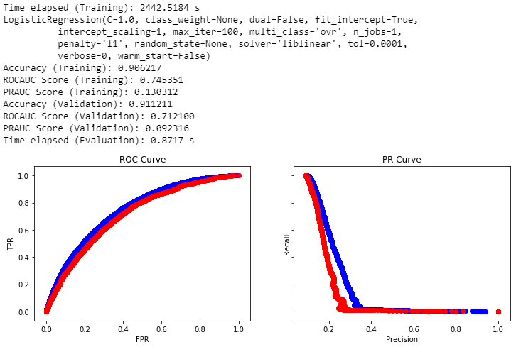
I started with data cleaning and data preprocessing, applied each of the ML model to the data, performed hyperparameter tuning to explore the potential of the models, and then analyzed the accuracy, Receiver Operating Characteristic (ROC) curves, and Precision-Recall (PR) curves and their respective Areas Under Curve (AUC) to evaluate the quality of the resulting models. As this dataset has highly unbalanced classes, ROCAUC or PRAUC are better metrics than the accuracy. I also applied different feature engineering techniques and compared the model performance. The detailed experiments and reports in the form of Jupyter notebooks are available on GitHub. I will also present some highlights here in this post.
Feature Discretization
The idea of using a hybrid model of decision tree ensembles and logistic regression comes from the paper Practical Lessons from Predicting Clicks on Ads at Facebook. In the paper, they trained gradient-boosted decision tree model and used it to perform feature discretization. The output (leaf node) of each tree is used as a categorical feature and an input to the logistic regression model. It is observed in the paper that this greatly helps the logistic regression model to take account of the nonlinearity and improve the accuracy metrics.
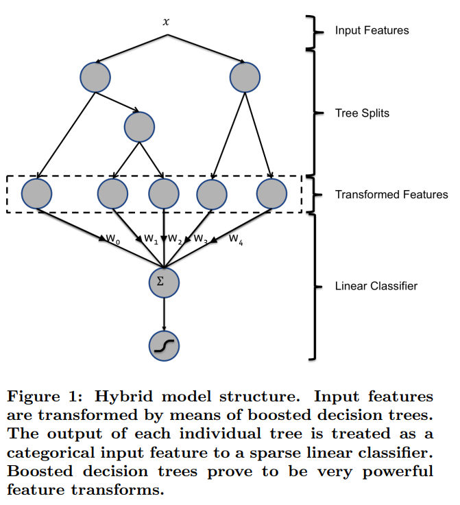
I experimented with two types of decision tree ensembles, Random Forests and Gradient-Boosted Decision Trees. For both methods, I limited the tree depth to 6 and the number of trees to 10. I used the best hyperparameters I found to train the models. I also tried using only the discretized features as the input to the logistic regression model, or using the discretized features concatenated with the original features.
For Random Forests, I extracted the decision path for each example from each tree. The decision paths are expressed as a vector of boolean values, indicating which subtree the decision path takes at each branch. These are used as the discretized features. The Random Forest model itself achieved an ROCAUC of 0.704 on the training set and 0.669 on the validation set. Using the discretized features alone, the best ROCAUC I obtained after hyperparameter tuning was 0.680 on the validation set. Using concatenated features, I got 0.714, slightly better than the best ROCAUC I got from using the original features, 0.713, and is the best ROCAUC I got in the entire series of experiments.
For Gradient-Boosted Decision Trees, I followed the Facebook paper approach more closely. I used the XGBoost implementation of gradient-boosted decision trees. I extracted the decision path’s leaf node for each example from each tree. The leaf nodes are expressed as integers, which can be treated as categorical features. I then performed one-hot encoding on these categorical features and used them as the discretized features. The ROCAUC obtained from the XGBoost model itself is 0.789 on the training set and 0.702 on the validation set. Using discretized features alone, the best ROCAUC I obtained is 0.701 on the validation set. Using concatenated features, the best I got is also 0.701.
Unfortunately, these techniques do not bring significant improvement on the model performance on this dataset as demonstrated in the Facebook paper. One hypothesis is that not many features have nonlinear relationships with the label.
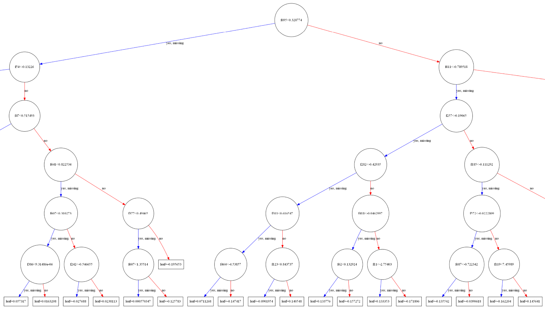
Please refer to LDP 08 - Feature Discretization with Random Forest.ipynb and LDP 11 - Feature Discretization with Gradient Boosted Decision Trees.ipynb for experiment details.
Feature Dimension Reduction
The dataset comes with 778 features and 105,471 entries. After performing one-hot encoding on categorical features, the number of features increased to 1,788, even more with feature expansion. For some ML models, it takes at least a few minutes or even up to hours to train on a personal computer. Therefore, I wanted to explore feature reduction techniques to reduce the number of features while retaining a high model performance. The techniques I tried are:
- Feature Hashing
- Feature Selection
- Principal Component Analysis (PCA)
- Decision Tree Feature Importance
For each technique, I set the target number of features k to be [1000, 500, 200, 100, 50, 20], selected the features, trained a Logistic Regression model with these features, and plotted the model accuracy, ROCAUC, and PRAUC to observe the trend of model quality as k decreases.
The first feature reduction technique I tried is feature hashing, also known as the hashing trick. Given a target number of features k, feature hashing uses a hash function to combine various original features into one column, resulting in a total of k columns. It usually works well for sparse features.
The second technique I tried is feature selection. Given the target number of features k and a scoring function, it will select the top k best-performing features with the highest scores. For this experiment, I used f_classif (ANOVA F-value) as my scoring function.
PCA is the third technique I applied. PCA transforms the features with a new basis that explains the most variance in the feature space. Selecting the top k principal components has a similar effect to selecting k best features, except that all features are mapped into a new space instead of remaining in the original form.
The last technique I tried is to use Decision Trees to perform feature selection. The importance of features is implied in the hierarchy of the tree. The sklearn.tree.DecisionTreeClassifier conveniently gives an importance score to each feature. I selected the k features with the importance scores.
For all four techniques, we can see that the ROCAUC gradually decreases as k decreases. The best ROCAUC occurs at k=1000, with values around 0.71. Interestingly, at k=20, feature hashing results in the lowest ROCAUC of 0.63, while decision tree feature importance results in the highest ROCAUC of 0.69, indicating that it preserved more information than the other three.
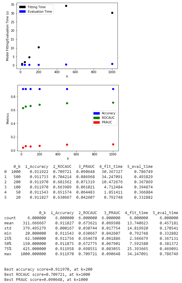
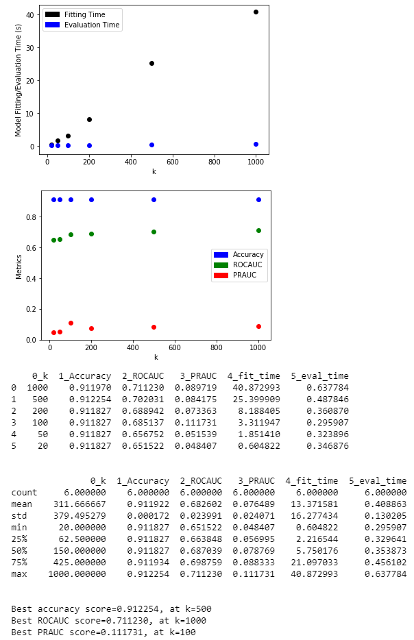


Please refer to LDP 04 - Feature Dimension Reduction.ipynb and LDP 06 - Feature Selection with Decision Trees.ipynb for experiment details.
Future Work Ideas
- Because I ran the experiments on a personal computer, I had limited computation power, and it limited my search techniques for the best hyperparameters. For example, if all experiments were done with 5-fold cross validation instead of just one, the hyperparameters selected would likely be better. I also tended to tune one hyperparameter at a time, but ideally it would be better to consider the interactions of hyperparameters and perform grid search or random search.
- The best results in terms of ROCAUC I obtained is from logistic regression. Theoretically speaking, logistic regression is a subset of neural networks because it consists of one single neuron, and I should be able to do better with neural networks. Due to the computation time required, I haven’t spent enough time to explore all possible architectures.
- Work on the original regression problem.

